Geometric distribution
| Table of contents | |
|---|---|
| - | Definition |
| - | Example |
| - | Expectation value |
| - | Variance value |
Definition
The geometric distribution is a discrete distribution
having propabiity
\begin{eqnarray}
\mathrm{Pr}(X=k) &=& p(1-p)^{k-1}
\\
&& (k=1,2,\cdots)
\end{eqnarray}
, where $0 \leq p \leq 1$.
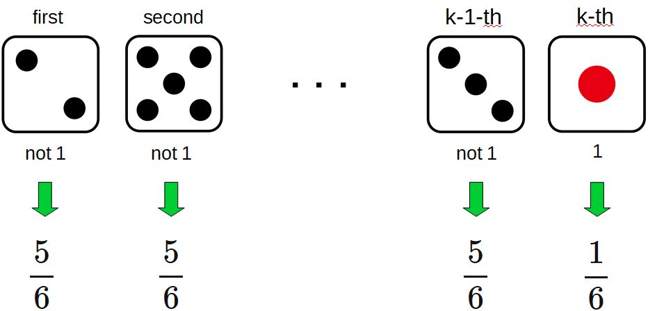
Example: Dice
We roll a cubic dice many times,
and let $X$ be the number of times until we roll a $1$.
The probability that $X = k$ obeys the geometric distribution for $p = \frac{1}{6}$,
\begin{eqnarray}
\mathrm{Pr}(X=k) &=& \frac{1}{6} \Big( 1- \frac{1}{6} \Big)^{k-1}
\\
&& (k=1,2,\cdots)
\end{eqnarray}
Explanation
Let $p$ be the probability rolling a $1$. Assuming that the cubic dice is symmetric without any distortion, \begin{eqnarray} p=\frac{1}{6} \end{eqnarray} The probability of rolling not $1$ is \begin{eqnarray} 1-p=\frac{5}{6} \end{eqnarray}
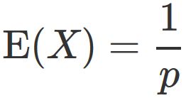
Expectation value
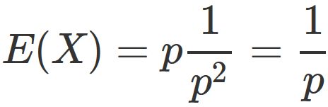
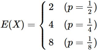
The expectation value of random variable $X$, if $X$ obeys the geometric distribution, is
Proof
Since $X$ obeys the geometric distribution, , the expectation value is
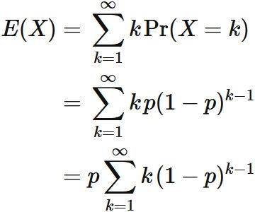
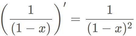
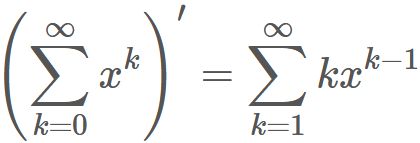
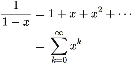
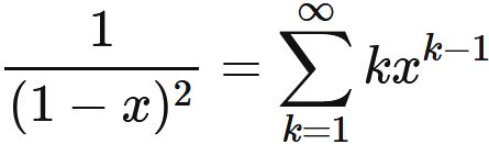
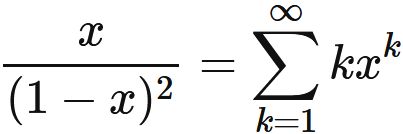
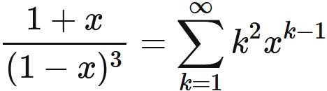
To find the sum in the right-hand side, we use Taylor expansion of function $1/(1-x)$,
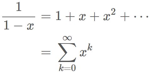
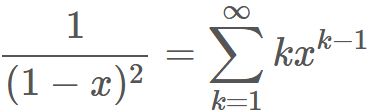
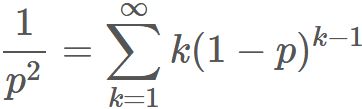
Substituting this into $(1)$, we obtain
Specific examples
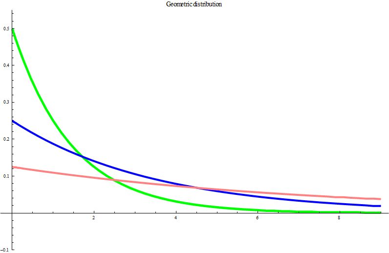
The figure below describes the geometric distribution for $p=\frac{1}{2}$ (green)、
, $p=\frac{1}{4}$ (blue)、
$p=\frac{1}{8}$ (pink).
Variance and Standard deviation
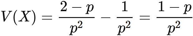
The variance and the standard devation of random variable $X$, if $X$ obeys the geometric distribution, are
\begin{eqnarray}
V(X) &=& \frac{1-p}{p^2}
\\
\\
\sigma(X) &=& \sqrt{V(X)}
\\
&=& \sqrt{\frac{1-p}{p^2}}
\end{eqnarray}
Proof
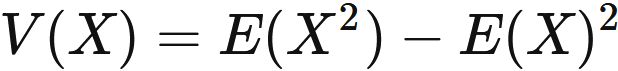
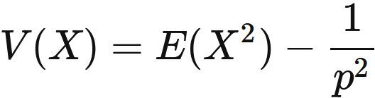
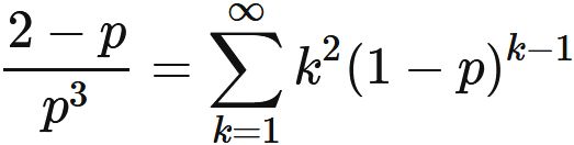
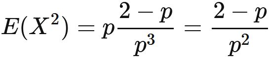
In general, the variance is the difference between the expectation value of the square and the square of the expectation value, i.e.,
Specific examples :
The figure below describes the geometric distribution for $p=\frac{1}{2}$ (green)、
, $p=\frac{1}{4}$ (blue)、
$p=\frac{1}{8}$ (pink).